Back to Software

Self-Expanding Convolutional Neural Networks

For this project, I worked with a team of three other students representing our university at the ProjectX North America competition. We developed a self-expanding convolutional neural network (SECNN) that starts small and grows during training only when the model detects that additional capacity would help. For context on the problem we were trying to solve, a regular convolutional neural network (CNN) is normally built by a developer deciding the number of layers and channels before training begins, and that architecture stays fixed. This can be an issue because a model that is too small may not learn enough while a model that is too large would waste memory and be computationally expensive. Oftentimes, developers have to train multiple different models with varying architectures before finding one that is suitable. Our SECNN addresses this issue by allowing the model to dynamically shape its own architecture depending on what it's being used for.

Read the paper here: Self Expanding Convolutional Neural Networks DOI: 10.48550/arXiv.2401.05686

Starting Architecture

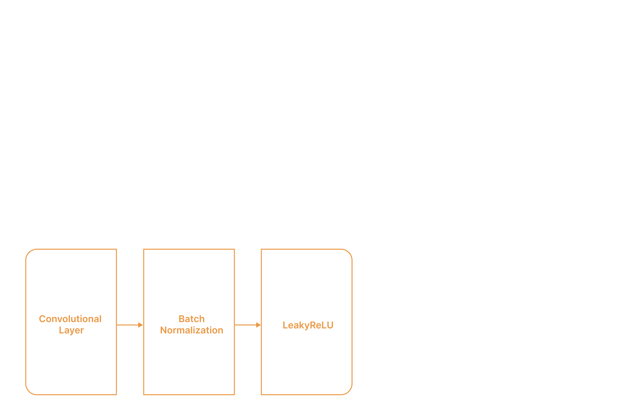
Our initial model contained three groups of image processing layers called convolutional blocks. Each block contained:

Convolutional Layer
Batch Normalization
LeakyReLU

A convolutional layer contains a small grid of numbers called a kernel that slides across an image (which is basically just a grid of pixel values) one section at a time.

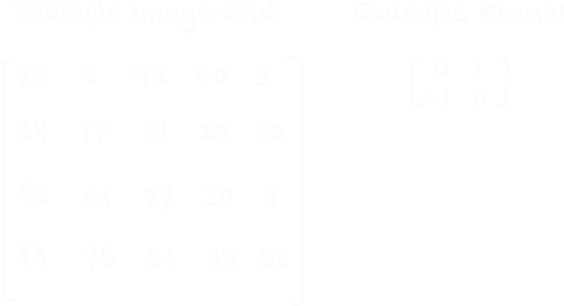
A convolution kernel moving across an image grid

At each position, it looks at the pixels underneath, multiplies the pixel values by its own grid values and adds it all together before storing it in a new grid. This new grid is called a channel, which can often detect patterns, edges, and corners of an image. The more channels, the more pattern detectors (wider CNN). Adding more convolutional layers can help with combining simple patterns learned from channels into more complicated features like textures, shapes, and parts of specific objects in the image (deeper CNN).

Batch Normalization rescales the output of the convolution layer by normalizing each output channel. This makes the values more stable to train with. Next, the LeakyReLU is an activation function that determines how much of a layer’s output continues on to the next stage. This is useful because it makes the network non-linear, meaning it can now learn more complicated patterns. We also added pooling layers after each convolutional block which reduces the size of feature maps and helps to prevent overfitting. We also had a skip connection from the first block to the final block in the network. This was important to include for our model as since new layers can be added during training, the network would become deeper and training would have to go through more and more layers during backpropagation and this can lead to the vanishing gradient problem, where the gradient becomes smaller as it passes through more layers and the first layer might receive barely any useful training signal to update its weights. This skip connection gives the network a shorter route so the earlier blocks are still able to be trained even as the architecture grows larger. The last part of our starting CNN contains a 1x1 convolution with a LeakyReLU activation to combine the extracted features from the previous layers. This is followed by a fully connected linear layer which converts these refined features into scores that can be used to determine the image’s class. Since we trained and evaluated our model using the CIFAR-10 dataset which has 10 possible image classes, the output layer produces 10 scores and the highest scoring class is the final prediction.

Starting self-expanding convolutional neural network architecture

Model Expansion during Training

The most important technical problem we addressed was determining when the model should expand. To do this, we used the natural expansion score:

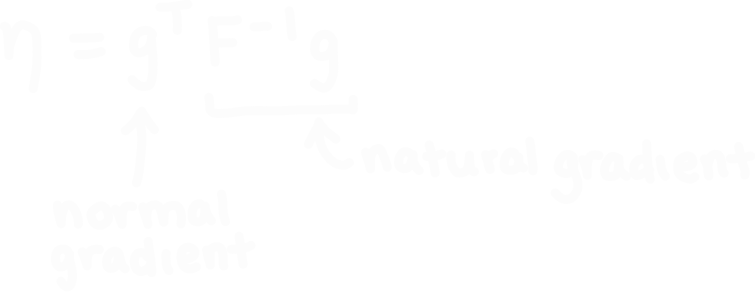
In the equation above: g is the normal gradient, and it tells us how changing each parameter affects the loss. It is transposed so that it can multiply with the next term. F^-1g is the natural gradient, this multiplies the inverse Fisher Matrix by g to adjust that gradient based on how sensitive the model’s predictions are to changes in certain parameters. The natural expansion score basically tells us how much potential the architecture has to reduce its loss if we follow the natural gradient direction. The larger the score, the more potential it has to reduce loss (which is good). We calculate the natural expansion score for our current architecture vs adding a layer vs adding a channel. Comparing these scores help the network decide whether to expand or not.

Important Note: F is the Fisher Information Matrix, which provides information about how sensitive a model’s predictions are to parameter changes. For example, if a network has parameters w1 and w2, a small change in w1 might significantly change the model’s final prediction while a change in w2 might barely affect it. The downside is that F can be HUGE because if our network has p parameters, F will have p x p values. So with e.g. 60,000 parameters, F will have 3.6 BILLION values which is extremely computationally expensive. To fix this, we used the Empirical Fisher Information Matrix:

Basically, while the full Fisher looks at how sensitive the model’s predictions are to parameter changes that are averaged over the probability distribution of data the model could potentially see (in plain terms, all kinds of data it could possibly encounter), the Empirical Fisher uses the actual training examples which significantly reduces the amount of calculations. To simplify it even further, we only looked at the diagonal of this Empirical Fisher Matrix which means we ignored interactions between different parameters and focused mainly on each parameter’s own sensitivity. While the Empirical Fisher had lots of benefits in terms of efficiency, it is less precise than actually using the full Fisher which is a limitation of our project. In the future, we could potentially go with a Kronecker-factored approximation (K-FAC) of the Fisher matrix which preserves more information about the relationship between parameters.

Ok so after some training, the model will calculate the current CNN’s natural expansion score. Then, we make a temporary copy of the network and the system tries adding a layer to each existing block. This newly added layer is an identity layer, which means it pretty much lets the information from the previous layer pass through without changing it much. This is better than adding a random convolutional layer because that could mix up the features when the information passes through it, and we want the model to be able to expand without having to restart training. Note that we did add a small amount of Gaussian noise to the identity layer so that it wasn’t a perfect copy. After this, we calculate the natural expansion score for each temporarily adjusted network and select the layer addition that gives the highest score.

Separately, the network temporarily adds output channels to the layers for every block. It again calculates the natural expansion score for each change and selects the highest one. Another problem we addressed when figuring out if and where to expand is to penalize expansions that are too large. For example, if temporary network 1 adds 2000 parameters and temporary network 2 adds 100,000 parameters, then network 2 will likely have a higher score because of its extra capacity. This defeats the purpose of our project since we wanted to avoid the model from getting unnecessarily large. So we modified our natural expansion score to take into account the cost of adding more complexity, and introduced a penalty for larger expansion:

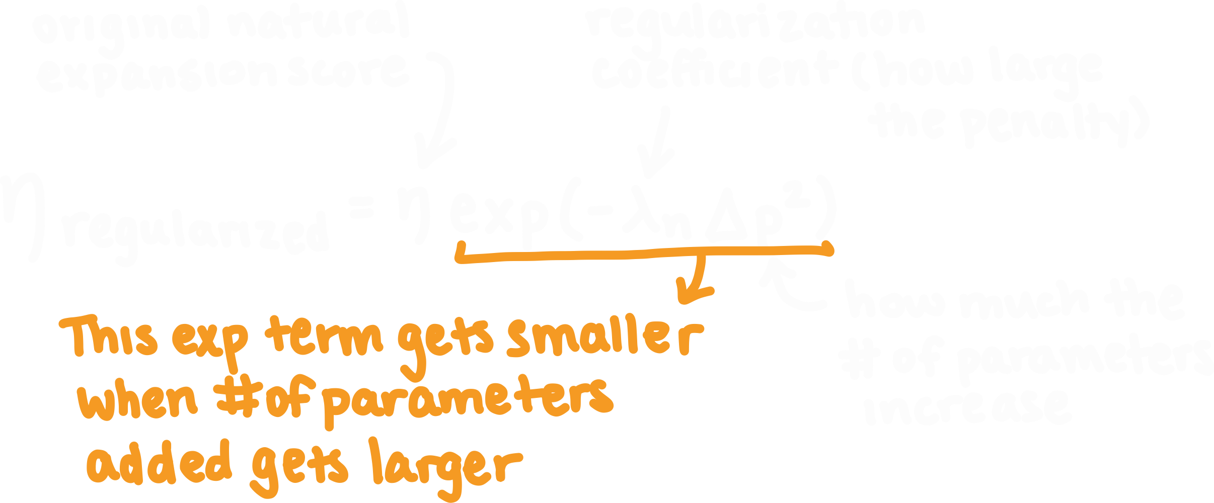
Regularized natural expansion score equation

Once we have the three regularized scores (the current model score is not regularized since delta p = 0 as no new parameters are added), we need to compare them to a threshold to decide whether to expand or not. In our code, we set tau = 2 as the expansion threshold. The next examples show how we determine whether to add a layer, channels, or perform no expansion at all.

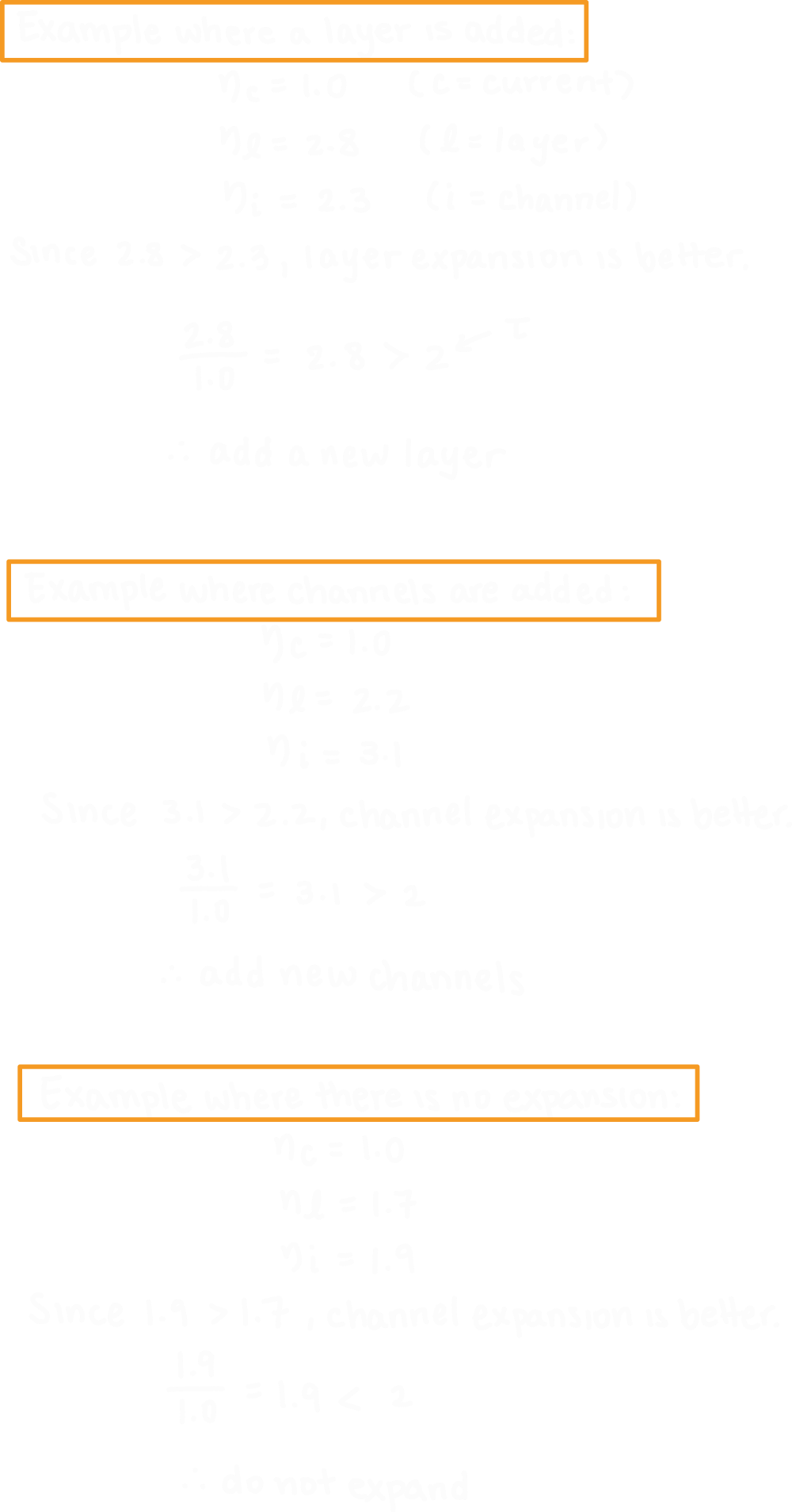
Once we decide to expand, we can now add the layer or channel to the real model. If channels are added, the next block also has to be adjusted since if Block 2 normally has a 16 channel output then Block 3 will expect 16 input channels. If we expand Block 2 to 20 channels then the input of Block 3 must also be expanded to match. After making this change, we continue with training as normal (we do not restart). We included a 10 epoch cooldown after an expansion to let the newly added layers/channels train and allow the network to stabilize before we ask whether we should change the architecture again. Of course, this could theoretically still expand forever so each block had a maximum capacity of N which we set to 10 to prevent uncontrolled growth.

Training and Evaluating the Model

We tested our model on the CIFAR-10 dataset, which contains 60,000 color images that fall into one of 10 categories: airplanes, automobiles, birds, cats, deer, dogs, frogs, horses, ships and trucks.

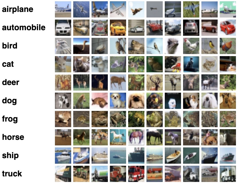
Each class had 6000 images with 5000 used for training and 1000 used for testing. We chose this dataset because it had a lot of images for training while keeping them lower resolution which decreased the computational cost. Each initial block used 16 outputs before expansion, and we used an NVIDIA GeForce RTX 3090 GPU to run the trials. We ran 5 separate trials which ran for 300 epochs each and the model processed groups of 512 images at a time. We set the learning rate to 0.002 and if validation accuracy did not improve after 15 epochs, then we would cut the learning rate in half. This is useful because later in the training process smaller adjustments will be more practical than taking large steps. We used cross-entropy loss to measure the performance of our predictions. Finally, to prevent overfitting we used three main methods: dropout, L1 regularization, and data augmentation.

We used 0.10 dropout for convolutional layers and 0.05 for the fully connected layers. This means that during a training pass, we would randomly disable 5-10% of the activations so the model doesn’t become overly dependent on certain neurons to make decisions. The small dropout rate we chose was good for our model because our starting network was quite small already. We also used L1 regularization, which is where the model is penalized for using weights that are unnecessarily large. Weights that are larger can make a model sensitive to tiny details in the training data, for example if it applies a large weight to bright corner pixels being correlated with cat images, it can overfit and make incorrect assumptions. We also augmented the data by randomly flipping training images horizontally to create more examples so that the network doesn’t memorize a specific image arrangement to make its decision.

Results

Out of the five trials we ran, the highest mean validation accuracy was 84.1%. At this accuracy, the models used an average of 62,698.4 parameters. These trials also showed how the model performed at smaller checkpoints, for example the five models only needed an average of 33,655.2 parameters to reach 80% validation accuracy, with the smallest one requiring only 22,636 parameters to reach 80%. When we compared this 80% checkpoint model with a ResNet-8 baseline, our SECNN used less than half as many parameters with its accuracy being only 6 percentage points lower.