Bellcrank Geometry Optimization

Problem

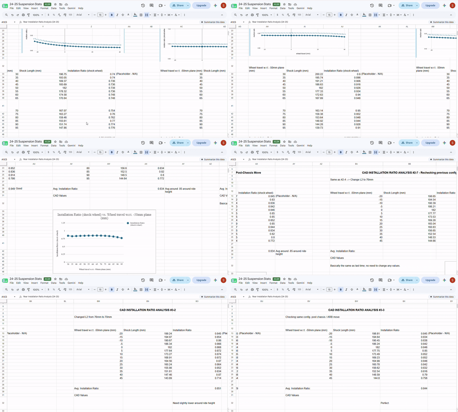
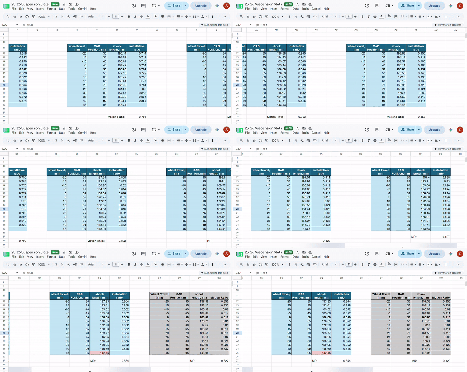
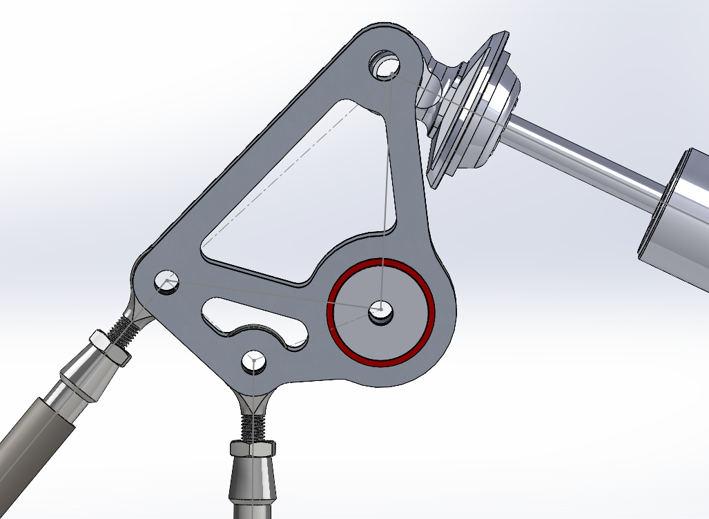
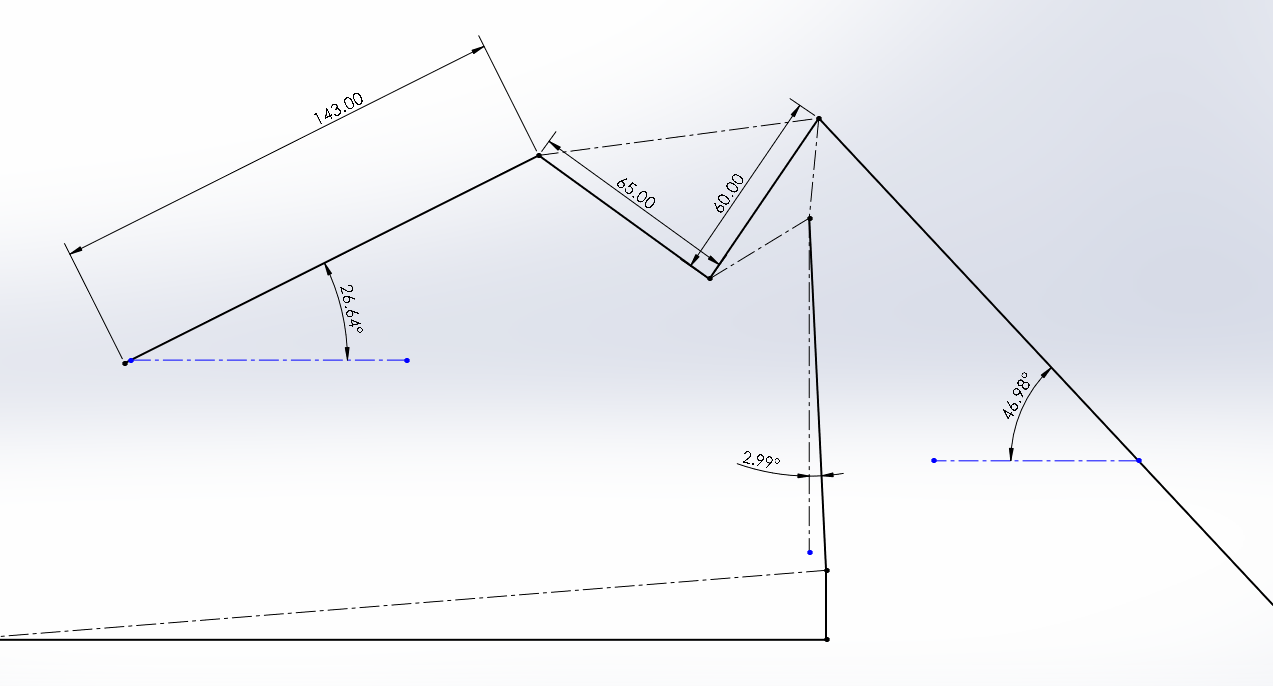
For many years, our formula electric team has bestowed one new suspension team member the task of optimizing the geometry of the bellcranks. While the project initially sounds fun, it is actually an incredibly tedious, time-consuming and monotonous task. I can say this because I was tasked with this project during my first year on the team. Now the reason why this takes forever is because the strategy that has been passed on year after year is to simply brute force as many geometry combinations as possible, run through a 14 position sweep on the parametric models in SolidWorks, and note down each value one by one. Surely we would have found a faster way to do it by now! You're wrong. I spent ten hours and pulled an all-nighter just to run through eleven geometries. I knew after that I had to find some way to automate this process. I thought it would be a fun challenge and would teach me some new SolidWorks skills, and hopefully save some of the future suspension members some precious time. I mean just look at this:

Automation Solution

Remember when I said it took me ten hours to run through eleven geometries? This script I wrote can now run through 920 geometries per bellcrank in only five hours. It also found a better geometry than I did.

Baseline Test

This test is done on the current bellcrank geometry, and it’s mainly to check that the macro is working and rebuilding properly. It runs the single geometry once through the entire 14 suspension positions in 5mm increments from 30 to 95mm of wheel travel (in CAD).

↓

Stage 1: Global Halton Screening

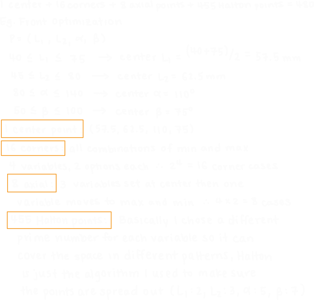
In the first stage, 480 different geometries are tested. For each geometry, the macro runs through 7 suspension positions (30, 40, 50, 60, 70, 80, 95) to get a broad idea of its motion ratio. It looks through the entire search space, using Halton sampling to select a wide range of geometries to test. I wrote down how these 480 geometries are chosen below.

↓

Stage 2: Regional Screening

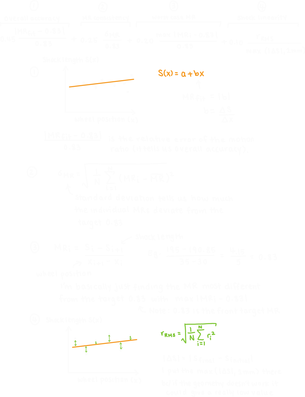
In this stage, the script will rank geometries from stage 1 that were successful. It uses the following motion ratio error term to determine the best geometries.

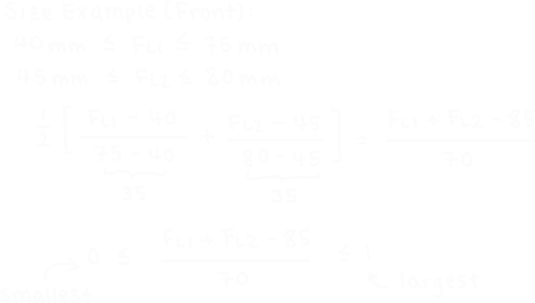
It also separately considers the size of the bellcrank, which we also want to minimize to reduce cost. I included how this is calculated below. I decided to consider the motion ratio score and size score independently because I didn’t want the algorithm to prefer a smaller bellcrank with a bad motion ratio. I made it so that we only consider the size for the bellcranks that have optimal motion ratio scores.

Based on these scores, stage 2 chooses the top 12 geometries. Since I still wanted to cover a broad range with this stage, I calculated the normalized distance between each pair of geometries just to make sure that they are far enough apart from each other (d ≥ 0.1) and we’re not concentrating our efforts on a single area of the graph just because the best 12 from stage 1 happen to be in the same place. This is how I did the normalization:

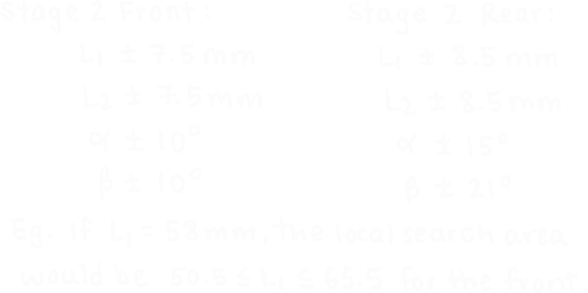
At each anchor, the search looks through a small area around it. Here’s an example of what I mean:

Overall, stage 2 went through 320 total geometries and each one was checked at all 14 suspension positions (30, 35, 40, 45, 50, 55, 60, 65, 70, 75, 80, 85, 90, 95).

↓

Stage 3: Fine Refinement

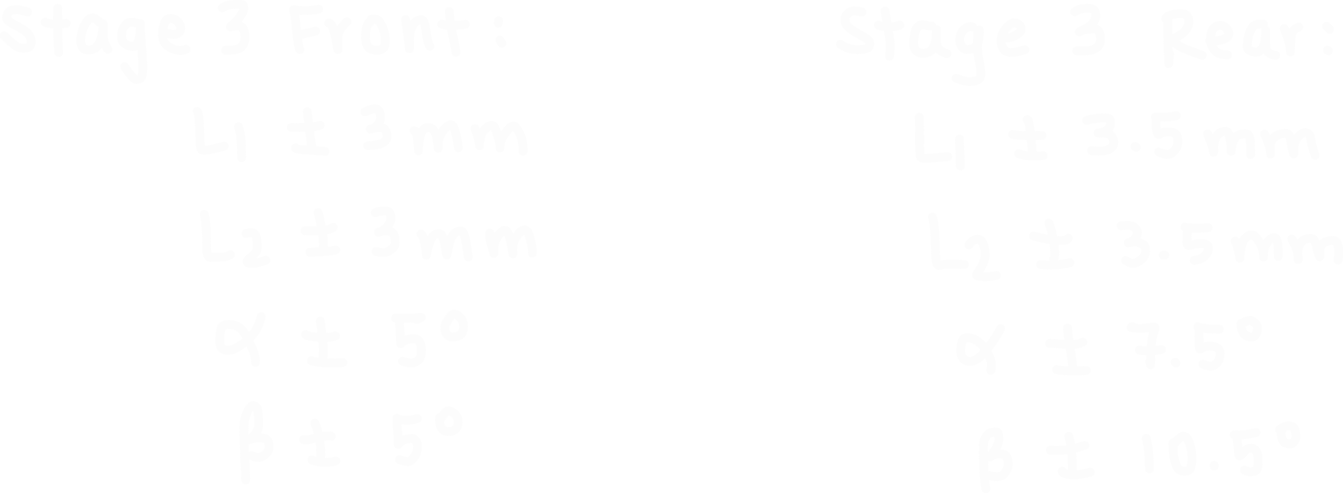
This is pretty much the same as step 2, except it chooses 8 anchors from stage 2 with a much smaller normalized distance requirement (d ≥ 0.04). It looks at a total of 120 geometries and goes through the full 14 position sweep with each one. The search space around each anchor is smaller in stage 3:

Below is a 14-second video rendition of the entire five hour process I described above. I made this on MATLAB using actual data from the solidworks optimization. The main takeaway is that the algorithm covers a wide range of geometries before narrowing the search toward the best one.

Loading macro...

These videos show the macro in action. It selects the geometry, applies it to the driver file, then rebuilds the dynamic suspension parametric model and runs through the different positions. Seeing this automatically do the same work I had previously spent ages doing by hand nearly brought tears to my eyes.

In total, 1840 geometries were tested (920 for the front and 920 for the rear). Each successful geometry was mainly ranked based on how closely their motion ratio curves followed the target value throughout the entire wheel travel. I considered both RMS error and the total motion ratio range to prevent a curve from getting a good ranking if it had a good average but big fluctuations. We needed the MR curve to be almost linear. The size of the bellcrank was also considered but only for geometries that had good MR behavior, and I used L1 + L2 as the measurement for overall size. Below are the top ten geometries found using my algorithm for the front and rear:

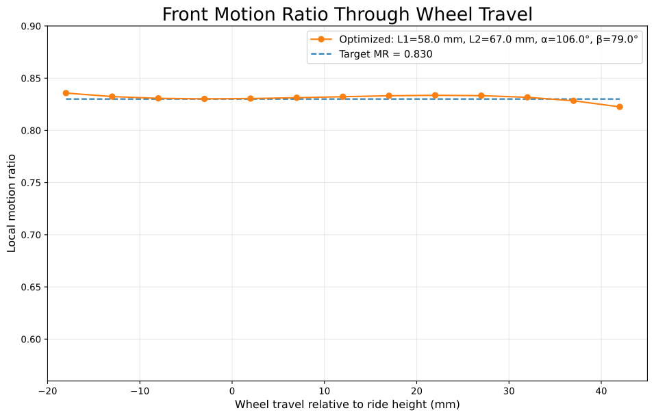
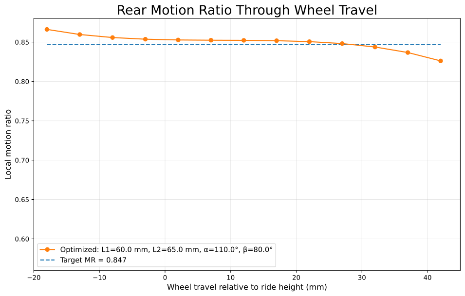
When I plotted the motion ratio curve for the highest ranking geometries in the front and rear, you can see that they are both pretty linear. The rear one does deviate slightly near the wheel travel limits, but its overall error is low and the damper is not expected to reach full compression or extension, which makes these extreme positions less significant when evaluating performance. I would consider these curves to demonstrate very good behavior.

The optimization script measured kinematic performance, but I still needed to verify that the physical bellcrank would be able to go through the entire 57mm of wheel travel without hitting a rod end or the damper. I applied the top geometries to our kinematic model and set it at both limits of wheel travel, making sure there was clearance on each side. I’m including this step because while scripts can automate a lot of the design process, forgetting to check whether something can physically work will be a pain later on if you just start manufacturing based on the geometry given to you by the script.

Force Calculations

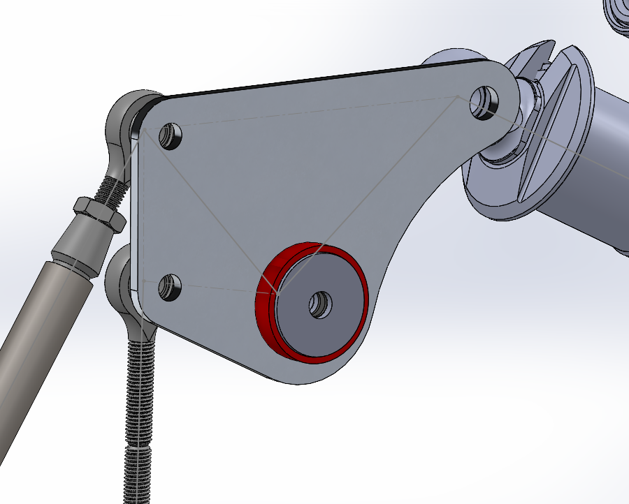
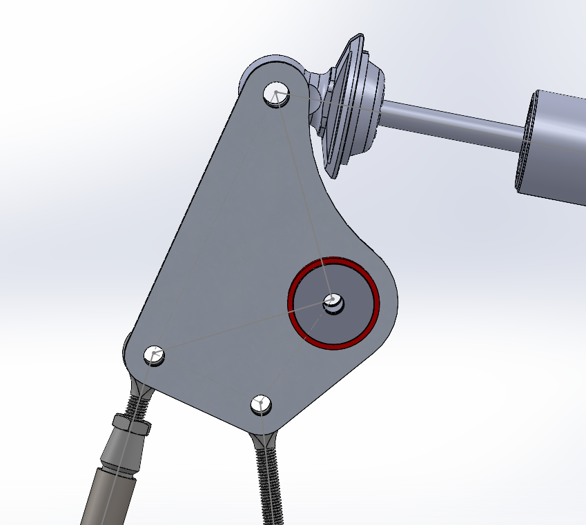
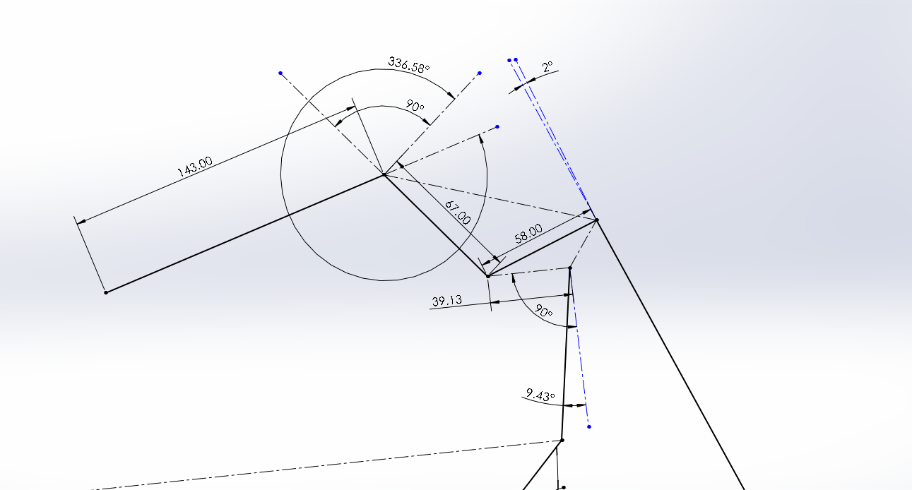
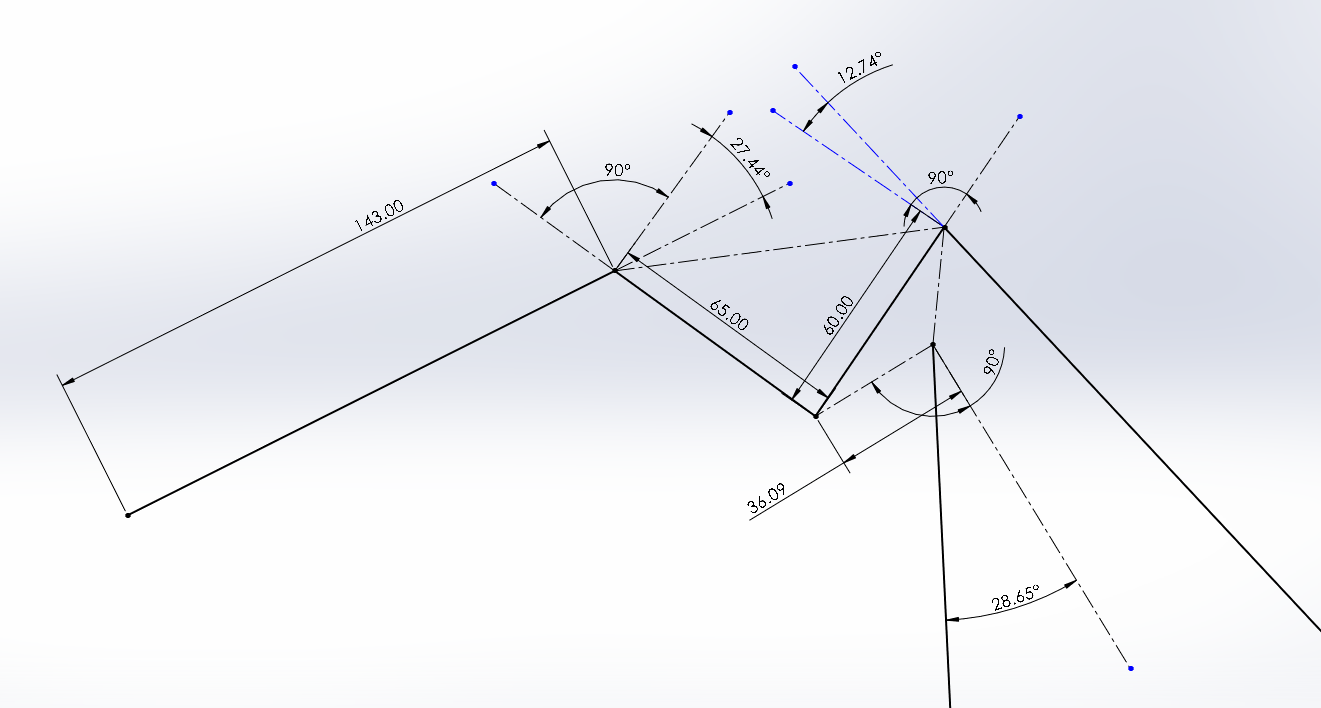
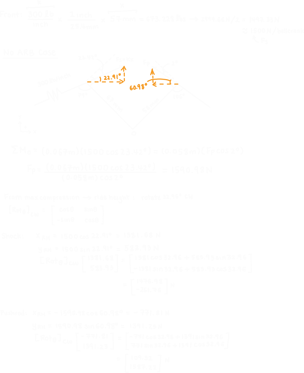
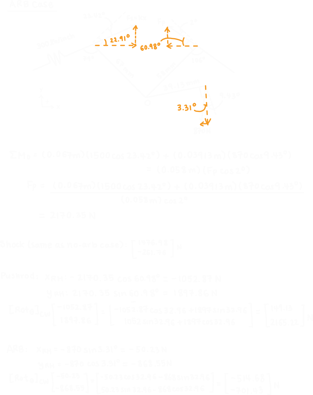
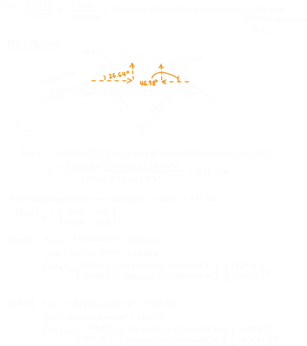
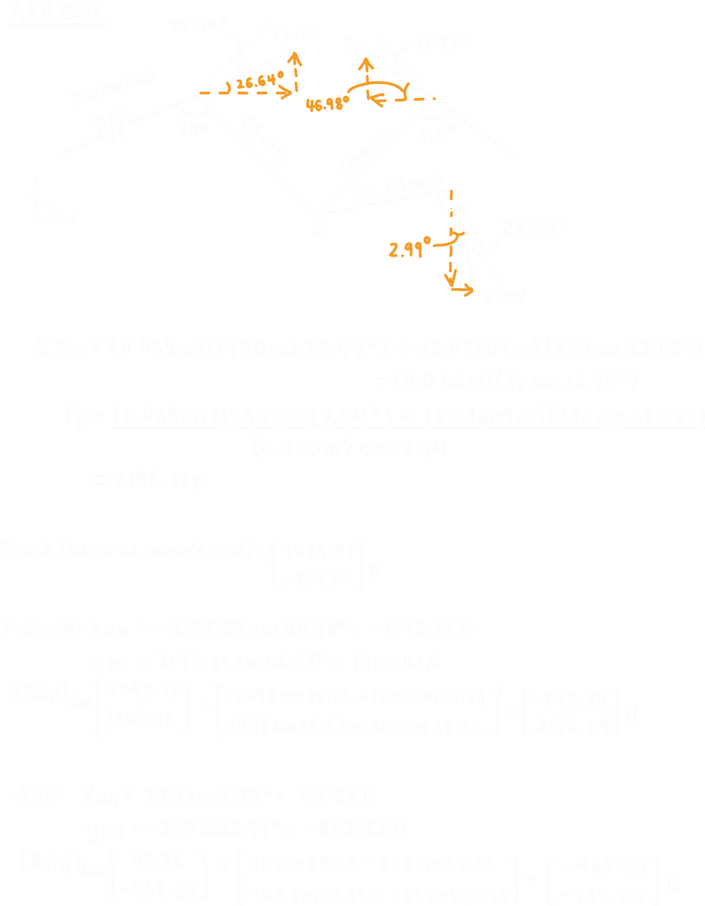
After finalizing the geometry, I calculated the forces needed to do a structural analysis. The next four images show you the dimensions I took from both the max compression case and the transformed case. The first two images show the front and rear assemblies at max compression, where I used the lever arm lengths and force angles at this position to calculate the pushrod force using a moment equilibrium around the bellcrank pivot.

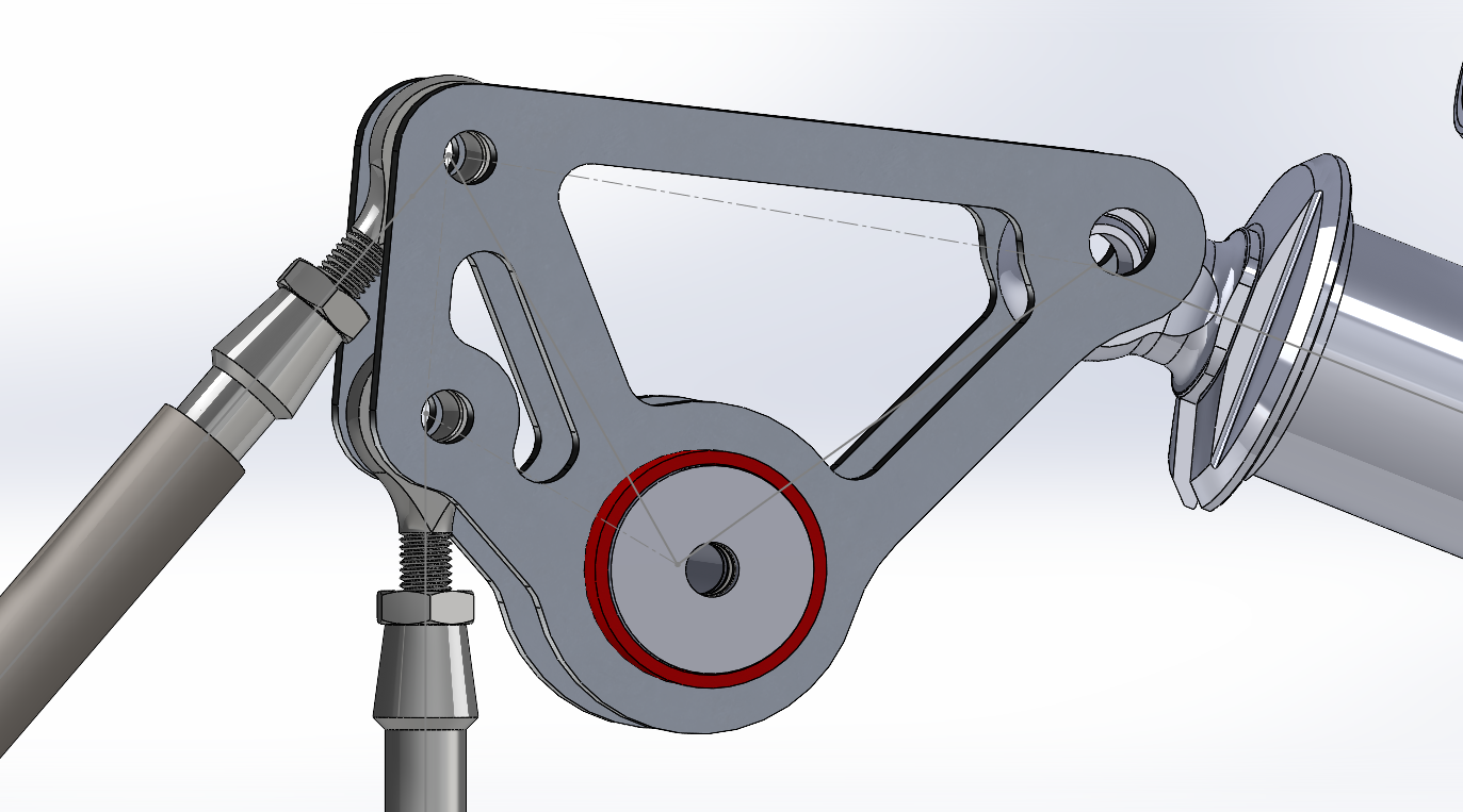
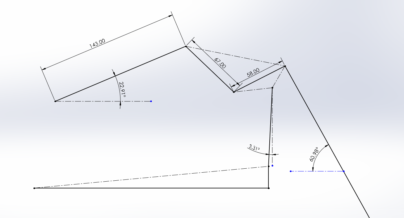
The next two images show the bellcranks rotated back to ride height. Since the force calculations were done when the suspension was at max compression, I had to use a rotation matrix to transform the force vectors back into the coordinate systems that would be used by ANSYS.

ANSYS FEA and Topology Optimization

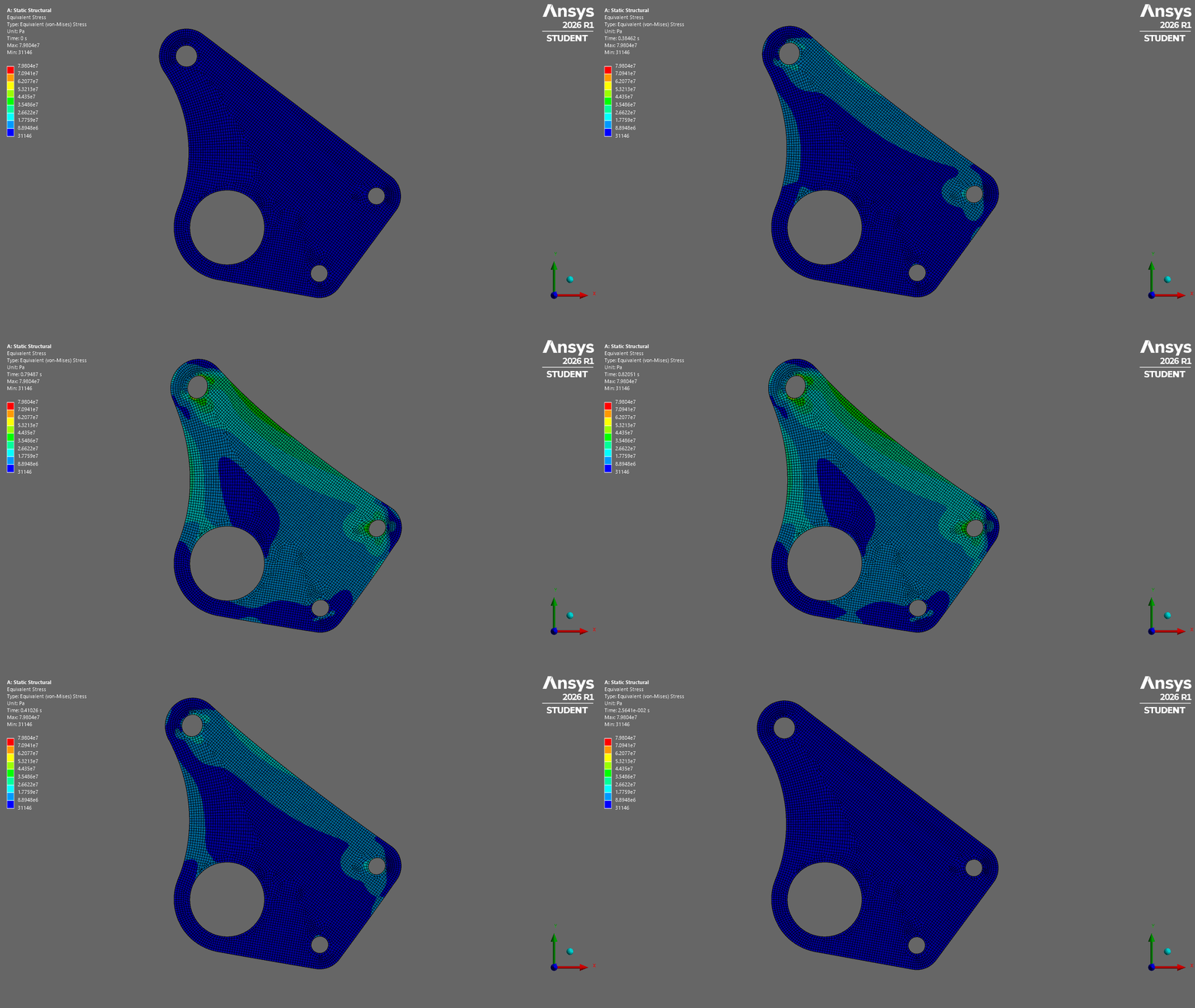
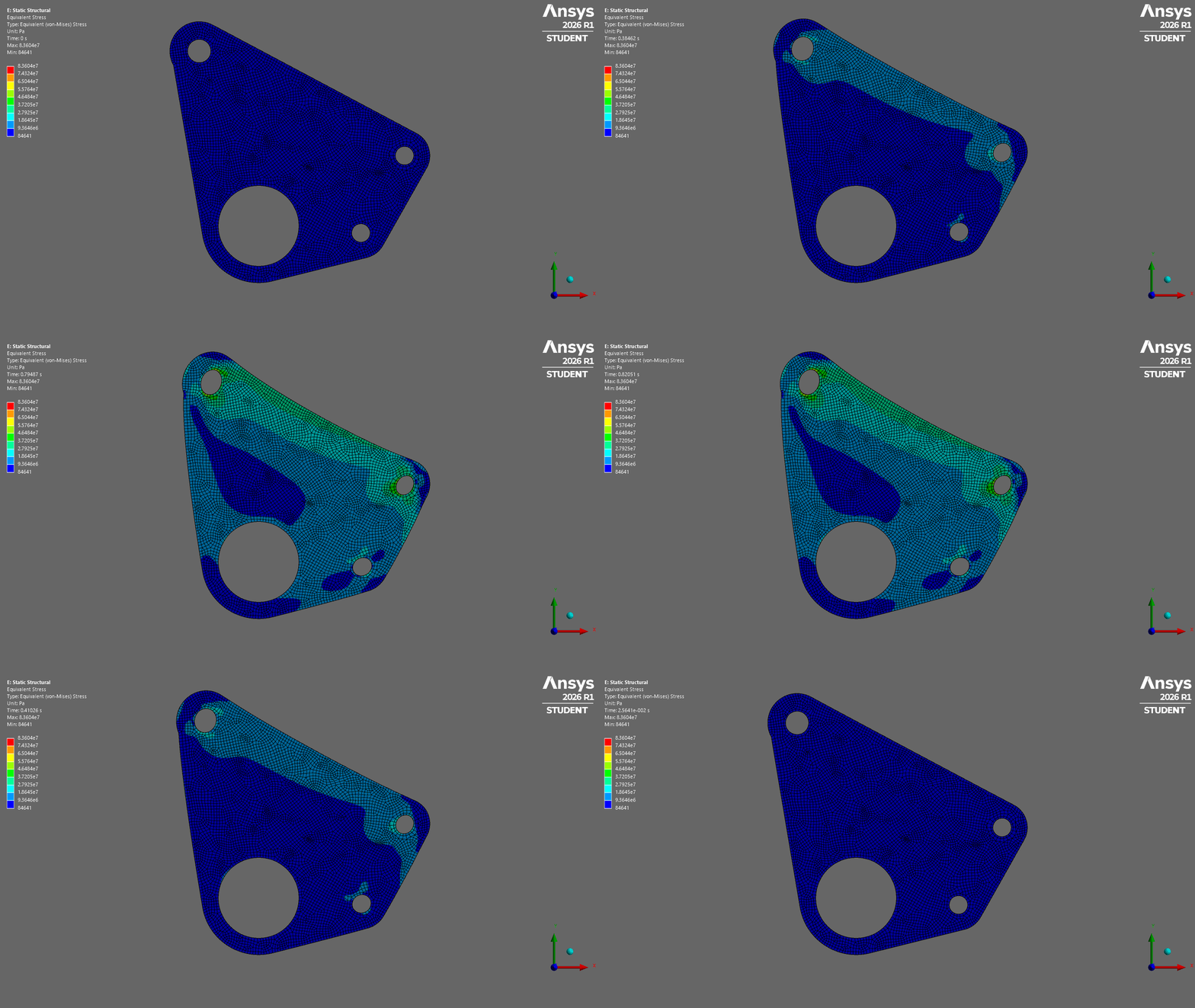
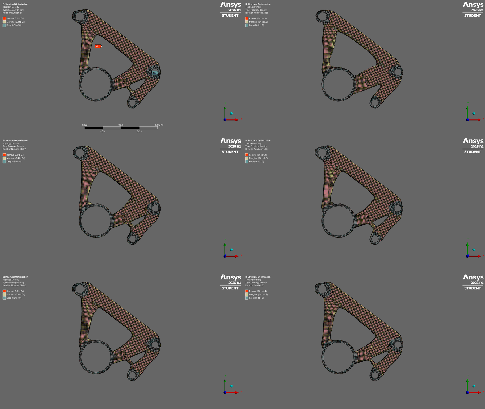
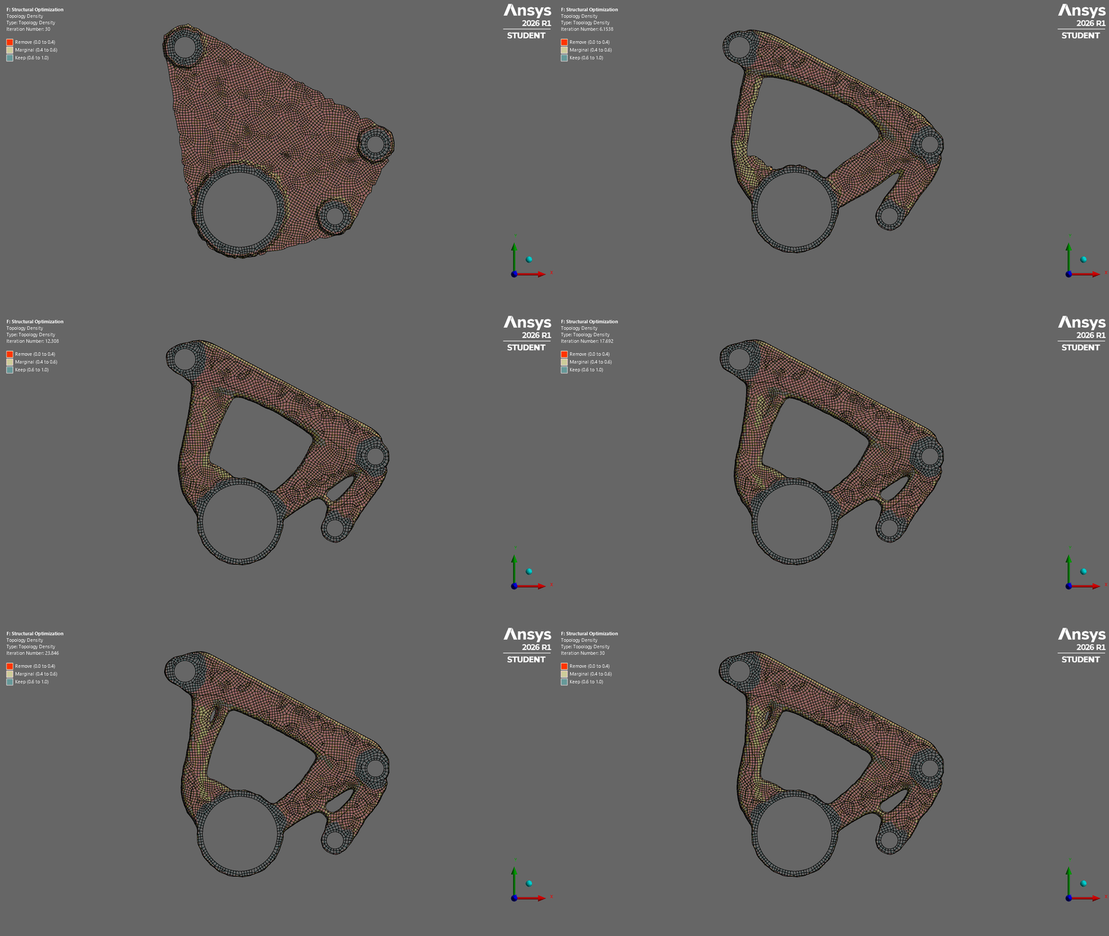
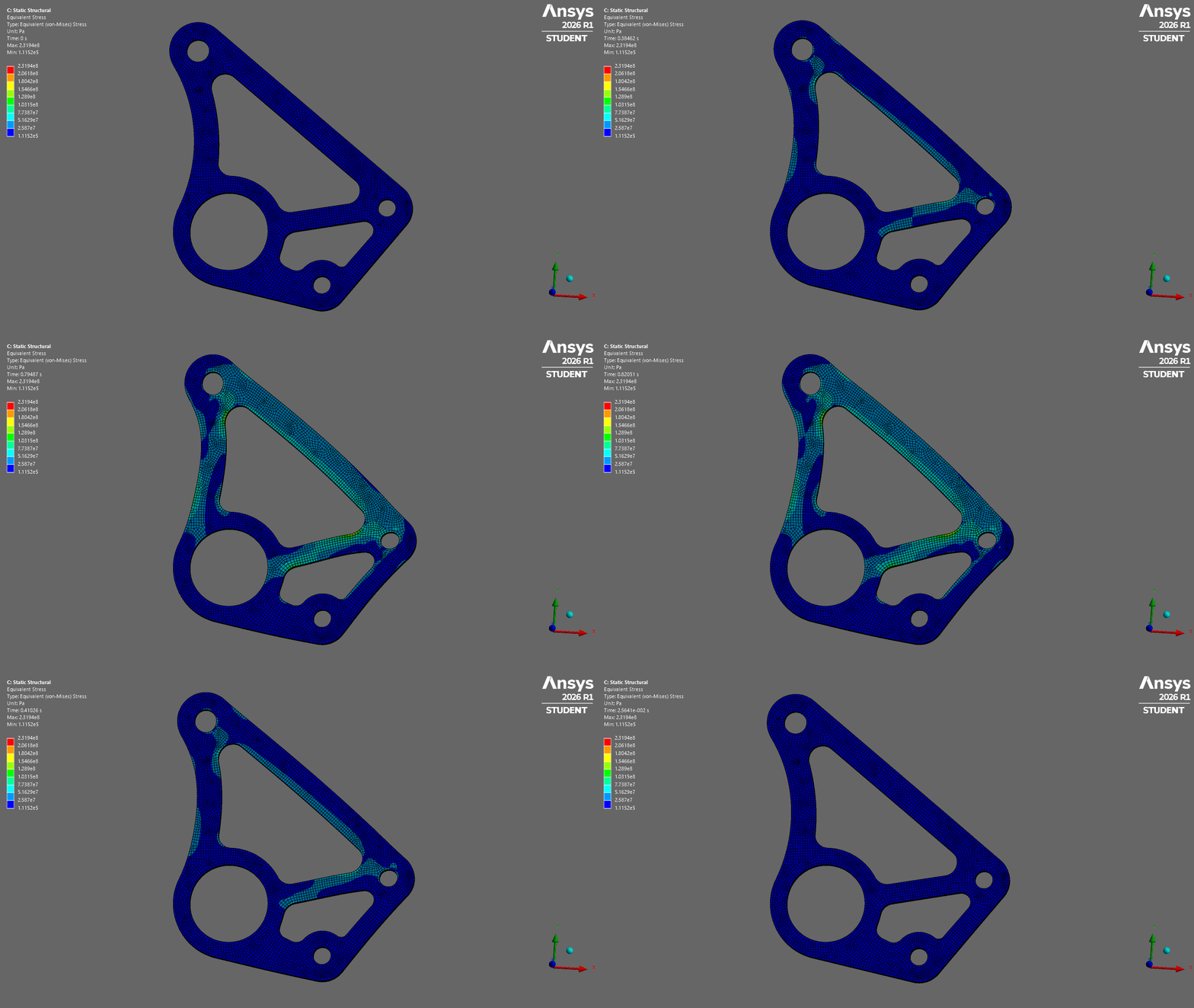
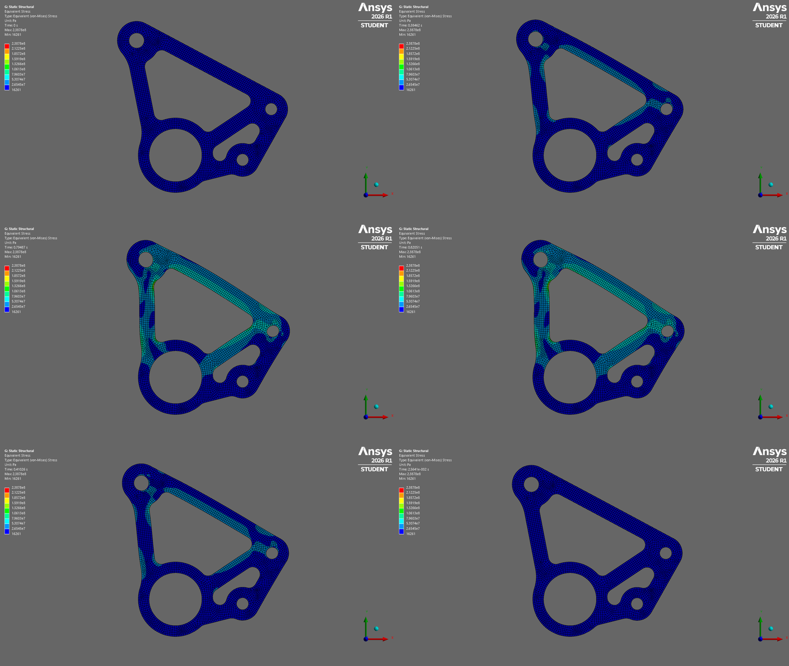
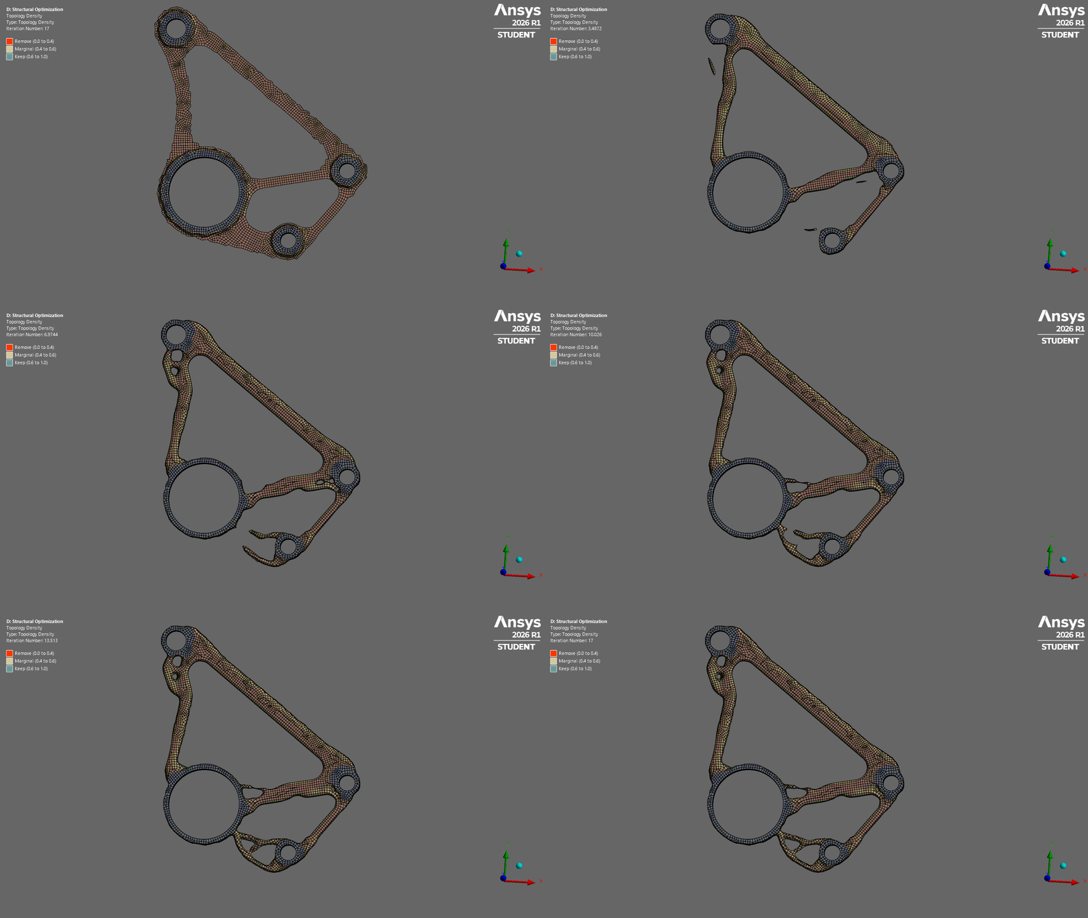
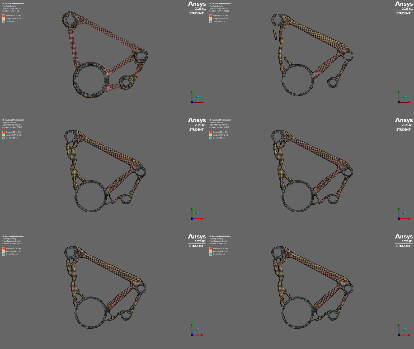
I first analyzed fully solid bellcranks to see how the stress distribution looks and identify the primary load paths between the pushrod, shock, central bearing and ARB connections. From this, I found that the central regions of the plate were receiving relatively little stress. After confirming this through topology optimization, I removed the excess material and conducted another structural analysis on the revised designs. For the front bellcrank, the ARB case had a maximum stress of 271.47 MPa and a safety factor (SF) of 1.70. The no-ARB case reached 231.94 MPa and had a SF of 1.99. For the rear, the no-ARB case reached 238.78 MPa with a SF of 1.93, while the ARB case reached 235.98 MPa with a SF of 1.96. All cases had a safety factor at or above 1.70, which showed that removing the material could reduce the plate’s mass while keeping its strength.

Final Design

Bellcrank engineering drawings

Front Bellcrank Rear Bellcrank Plate Rear Bellcrank Assembly

Manufacturing

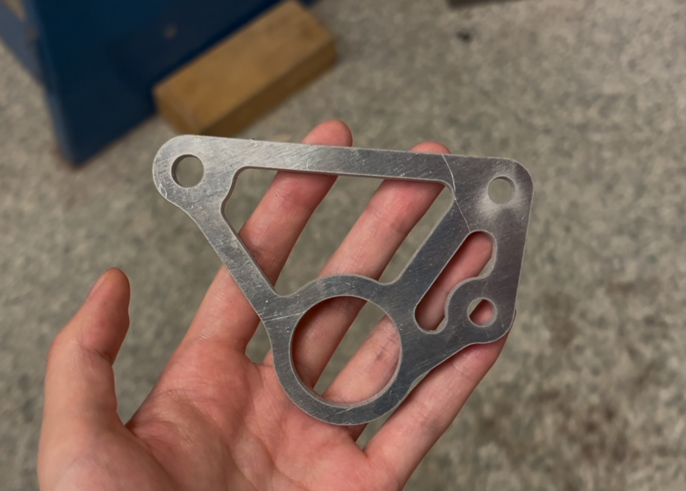
The final bellcrank was manufactured from 3.18mm thick 7075-T6 aluminum using a waterjet cutter.